Matrix multiplication
This guide demonstrates how to use Kernel Tuner to test and tune kernels, using matrix multiplication as an example.
Matrix multiplication is one of the most well-known and widely-used linear algebra operations, and is frequently used to demonstrate the high-performance computing capabilities of GPUs. As such, matrix multiplication presents a familiar starting point for many GPU programmers.
Note: If you are reading this guide on the Kernel Tuner’s documentation pages, note that you can actually run this guide as a Jupyter Notebook. Just clone the Kernel Tuner’s GitHub repository. Install using pip install .[tutorial,cuda] and you’re ready to go! You can start the notebook by typing “jupyter notebook” in the “kernel_tuner/doc/source” directory.
Make sure to execute all the code cells you come across in this tutorial by selecting them and pressing shift+enter.
Naive CUDA kernel
We’ll start with a very simple kernel for performing a matrix multiplication in CUDA. The idea is that this kernel is executed with one thread per element in the output matrix. As such, each thread \((i,j)\) iterates over the entire row \(i\) in matrix \(A\), and column \(j\) in matrix \(B\).
To keep the code clean and simple, we’ll assume that we only work with square matrices. Execute the following cell to write our naive matrix multiplication kernel to a file name “matmul_naive.cu” by pressing shift+enter.
[ ]:
%%writefile matmul_naive.cu

#define WIDTH 4096

__global__ void matmul_kernel(float *C, float *A, float *B) {
    int x = blockIdx.x * block_size_x + threadIdx.x;
    int y = blockIdx.y * block_size_y + threadIdx.y;
    float sum = 0.0;

    for (int k=0; k<WIDTH; k++) {
        sum += A[y*WIDTH+k] * B[k*WIDTH+x];
    }

    C[y*WIDTH+x] = sum;
}
This kernel assumes that the width and height of the matrices A, B, and C is equal to WIDTH, which is known at compile time. Of course, you’ll want a more flexible solution in reality, but this is just an example kernel to demonstrate how to use Kernel Tuner.
There are two more contants in the code that are currently undefined. These are block_size_x and block_size_y, these are the names that Kernel Tuner uses by default for denoting the thread block dimensions in x and y. The actual values used for these constants at compile time can be any sensible value for thread block dimensions. As long as we create enough threads to compute all elements in \(C\), the output will not be affected by the value of block_size_x and block_size_y.
Parameters in the code that have this property are called tunable parameters.
Because we can pick any value for these parameters, we can use auto-tuning to automatically find the best performing combination of parameters. That’s exactly what we’re going to do in this tutorial!
Tuning a naive kernel
Now we will have a look at how to use Kernel Tuner to find the best performing combination of tunable parameters for our naive matrix multiplication kernel. We’ll go over the process of creating an auto-tuning script step-by-step.
Because the tuner will need to execute the kernel, we start with creating some input data.
[ ]:
import numpy as np
problem_size = (4096, 4096)

A = np.random.randn(*problem_size).astype(np.float32)
B = np.random.randn(*problem_size).astype(np.float32)
C = np.zeros_like(A)

args = [C, A, B]
In the above Python code, we’ve specified the size of matrices and generated some random data for matrix \(A\) and \(B\), and a zeroed matrix \(C\). We’ve also created a list named args that contains the matrices C, A, and B, which will be used as the argument list by the tuner to call the kernel and measure its performance.
The next step is specifying to the tuner what values can be used for the thread block dimensions in x and y. In other words, we specify the tunable parameters and the possible values they can take.
[ ]:
from collections import OrderedDict
tune_params = OrderedDict()
tune_params["block_size_x"] = [16, 32, 64]
tune_params["block_size_y"] = [1, 2, 4, 8, 16, 32]
We are creating a dictionary to hold the tunable parameters. The name of the parameter is used the key, and the list of possible values for this parameter is the value for this key in the dictionary. We are using a small set of possible values here, but you are free to specify any values that you like. In general, we try to keep the total number of threads in a thread block as a multiple of the warpsize (32) on the GPU.
Also, to keep our kernel clean and simple, we did not include any bounds checking in the kernel code. This means that, for the kernel to run correctly, we need to make sure that the number of threads used in a particular dimension divides the size of the matrix in that dimension. By using 4096 as the width and height of our matrix and using only powers of two for our thread block dimensions we can avoid memory errors.
Before we start tuning, we will also tell Kernel Tuner how to compute a metric that we commonly use to express the compute performance of GPU kernels, namelijk GFLOP/s, which stands for giga floating-point operations per second. User-defined metrics are specified using the metrics option and should be supplied using an ordered dictionary, because metrics are composable.
[ ]:
from collections import OrderedDict
metrics = OrderedDict()
metrics["GFLOP/s"] = lambda p : (2*problem_size[0]**3/1e9)/(p["time"]/1e3)
Now that we’ve specified the input, the tunable parameters, and a user-defined metric, we are ready to call Kernel Tuner’s tune_kernel method to start auto-tuning our kernel.
[ ]:
from kernel_tuner import tune_kernel
results = tune_kernel("matmul_kernel", "matmul_naive.cu", problem_size, args, tune_params, metrics=metrics)
Before looking at the result, we’ll explain briefly how we called tune_kernel. The first argument is the name of the kernel that we want to tune. The second argument is a string that contains the filename of the kernel. It is also possible to directly pass a string that contains the code, or to pass a Python function that generates the kernel code. The tuner will figure out which language (CUDA or OpenCL) is being used in the kernel code. The third argument to tune_kernel is the problem
size, which is used by the tuner to compute the grid dimensions for our kernel. To compute the grid dimensions the tuner needs to know the thread block dimensions, which we have specified using the tunable parameters (fifth argument). The fourth argument is the argument list that the tuner will need to actually call the kernel.
As we can see the execution times printed by tune_kernel already vary quite dramatically between the different values for block_size_x and block_size_y. However, even with the best thread block dimensions our kernel is still not very efficient.
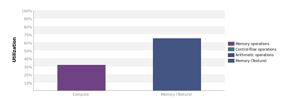
Therefore, we’ll have a look at the Nvidia Visual Profiler to find that the utilization of our kernel is actually pretty low:  There is however, a lot of opportunity for data reuse, which is realized by making the threads in a thread block collaborate.
Increase work per thread
A commonly used code optimization in GPU programming is to increase the amount of work performed by each thread. This optimization has several benefits. It increases data reuse within the thread block and reduces the number of redundant instructions executed by distinct threads. This code optimization is typically called 1xN Tiling or thread-block-merge. We will use two different forms of 1xN tiling in this example:
First of all, in the x-direction we will use tiling in a way that is similar to the convolution example (used as part of the ‘Getting Started’ tutorial). The area of output data that is processed by a single thread block is increased by a factor of N, and as such shared memory usage also increases by a factor \(N\). This means that the number of thread blocks needed to execute the kernel for this problem size is also reduced by a factor of \(N\). While this may reduce occupancy due to increased shared memory and register usage, this optimization drastically reduces the number of redundant instructions that were previously distributed across multiple thread blocks.
Secondly, in the y-direction we will use a different form of 1xN tiling, where we tile within the thread block. This too means that threads will compute multiple elements, but in this case, not the total number of thread blocks is reduced, but instead the number of threads per block goes down.
Note that these two different forms of tiling could have combined in different or even multiple ways to increase the tuning parameter space even further. However, for the purposes of this tutorial, the resulting kernel is already complex enough:
[ ]:
%%writefile matmul.cu

#define WIDTH 4096

__global__ void matmul_kernel(float *C, float *A, float *B) {

    __shared__ float sA[block_size_y*tile_size_y][block_size_x];
    __shared__ float sB[block_size_y*tile_size_y][block_size_x * tile_size_x];

    int tx = threadIdx.x;
    int ty = threadIdx.y;
    int x = blockIdx.x * block_size_x * tile_size_x + threadIdx.x;
    int y = blockIdx.y * block_size_y * tile_size_y + threadIdx.y;
    int k, kb;

    float sum[tile_size_y][tile_size_x];
    for (int i=0; i < tile_size_y; i++) {
        for (int j=0; j < tile_size_x; j++) {
            sum[i][j] = 0.0;
        }
    }

    for (k = 0; k < WIDTH; k += block_size_x) {

        __syncthreads ();
        #pragma unroll
        for (int i = 0; i < tile_size_y; i++) {
            sA[ty + block_size_y * i][tx] = A[y * WIDTH + block_size_y * i * WIDTH + k + tx];

            #pragma unroll
            for (int j = 0; j < tile_size_x; j++) {
                sB[ty + block_size_y * i][tx + j * block_size_x] =
                                    B[(k + ty + block_size_y * i) * WIDTH + x + j * block_size_x];
            }
        }
        __syncthreads ();

        //compute
        #pragma unroll
        for (kb = 0; kb < block_size_x; kb++) {

            #pragma unroll
            for (int i = 0; i < tile_size_y; i++) {
                #pragma unroll
                for (int j = 0; j < tile_size_x; j++) {
                        sum[i][j] += sA[ty + block_size_y * i][kb] * sB[kb][tx + j * block_size_x];
                    }
            }

        }

    }

    //store result
    #pragma unroll
    for (int i = 0; i < tile_size_y; i++) {
        #pragma unroll
        for (int j = 0; j < tile_size_x; j++) {
            C[y * WIDTH + x + block_size_y * i * WIDTH + j * block_size_x] = sum[i][j];
        }
    }

}
First of all we’ll need to expand our tune_params dictionary to include our newly introduced tunable parameters. We’ll choose a couple of small values for the tiling factors in both the x and y-dimension, to keep the search space manageable.
[ ]:
tune_params["tile_size_x"] = [1, 2, 4]
tune_params["tile_size_y"] = [1, 2, 4]
As explained in the text above, the tiling factors will reduce the number of thread blocks needed in their respective dimensions with a factor of N, where N is the tiling factor in that dimension. This is something that we will need to tell the tuner, otherwise it may execute the kernel with too many thread blocks.
We can tell the tuner how the grid dimensions need to be computed. So far, we’ve only used the default behavior of computing the grid dimensions by dividing the problem size with the thread block size in each dimension. However, the tuner now also needs to take the tiling factor into account. We specify this by setting up grid divisor lists, that will contain the names of all the tunable parameters that divide the grid in a particular dimension. These grid divisor lists will be passed as
optional arguments when we call tune_kernel.
[ ]:
grid_div_x = ["block_size_x", "tile_size_x"]
grid_div_y = ["block_size_y", "tile_size_y"]
Remember that the area operated on by the thread block should be a square. In this kernel however, we allow block_size_x and block_size_y to vary independently, while tile_size_y increases the amount of work per thread in the y-direction within the thread block. This yields a discontinuous search space in which only part of the configurations are actually valid. Therefore, we again use the restrictions= option of tune_kernel. After this, we are ready to call tune_kernel
again.
[ ]:
restrict = ["block_size_x==block_size_y*tile_size_y"]

results = tune_kernel("matmul_kernel", "matmul/matmul.cu", problem_size, args, tune_params,
                      grid_div_y=grid_div_y, grid_div_x=grid_div_x, metrics=metrics,
                      restrictions=restrict)
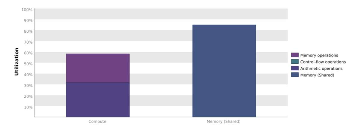
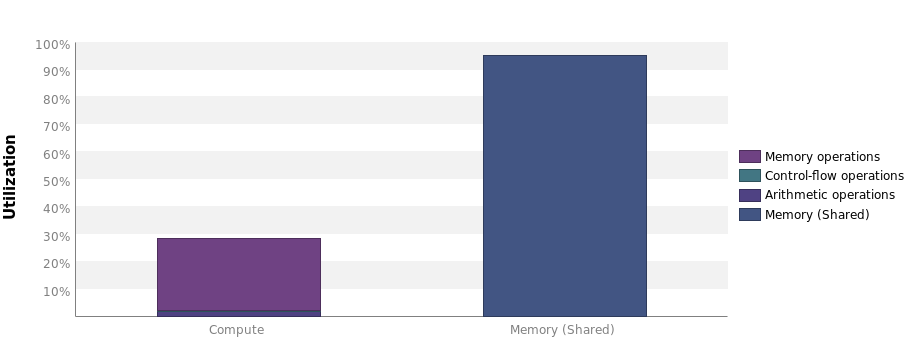
As we can see the number of kernel configurations evaluated by the tuner has increased again. Also the performance has increased quite dramatically with roughly another factor 3. If we look at the Nvidia Visual Profiler output of our kernel we see the following:

As expected, the compute utilization of our kernel has improved. There may even be some more room for improvement, but our tutorial on how to use Kernel Tuner ends here. In this tutorial, we have seen how you can use Kernel Tuner to tune kernels with a small number of tunable parameters, how to impose restrictions on the parameter space, and how to use grid divisor lists to specify how grid dimensions are computed.
